5  Data processing

As a useful starting point, Revol et al. (2024) propose a five-step framework, with an accompanying R package (esmtools) and tutorial website for pre-processing ESM data: (1) import and preliminary checks, (2) verify the design and sampling scheme, (3) examine response behaviour, (4) compute and transform variables, and (5) describe and visualise. This chapter follows those steps with plain dplyr code so that each operation is visible. The data come from the simulation in Appendix A.

5.1 Data structure

Analysis-ready ESM data are in long format: one row per scheduled prompt per participant, including prompts that were not answered. Keeping unanswered rows is necessary for computing compliance, for building lags correctly, and for modelling missingness.

Column	Meaning	Notes
id	Participant identifier	Level-2 unit
day	Study day (1, 2, …)	Based on the participant’s own start date, not the calendar
beep	Prompt number within day (1–6)	Scheduled position, not the count of answered prompts
scheduled	When the prompt was scheduled or sent	With time zone
started, completed	When the questionnaire was opened and submitted	NA if not answered
stress, na_*	Momentary responses	Level-1 variables
neuro	Baseline trait score	Level-2 variable, repeated on every row

library(dplyr)
source("R/simulate_esm.R")   # defines simulate_esm(); see Appendix A

esm <- simulate_esm()
glimpse(esm)

Rows: 8,400
Columns: 12
$ id           <int> 1, 1, 1, 1, 1, 1, 1, 1, 1, 1, 1, 1, 1, 1, 1, 1, 1, 1, 1, …
$ day          <int> 1, 1, 1, 1, 1, 1, 2, 2, 2, 2, 2, 2, 3, 3, 3, 3, 3, 3, 4, …
$ beep         <int> 1, 2, 3, 4, 5, 6, 1, 2, 3, 4, 5, 6, 1, 2, 3, 4, 5, 6, 1, …
$ scheduled    <dttm> 2026-03-02 09:48:00, 2026-03-02 11:28:00, 2026-03-02 15:…
$ started      <dttm> 2026-03-02 09:51:04, 2026-03-02 11:32:25, 2026-03-02 15:…
$ completed    <dttm> 2026-03-02 09:51:38, 2026-03-02 11:32:54, 2026-03-02 15:…
$ neuro        <dbl> 0.5205891, 0.5205891, 0.5205891, 0.5205891, 0.5205891, 0.…
$ stress       <dbl> 41, 44, 38, 32, 42, 47, 80, 62, 65, NA, 71, 56, 37, 17, 3…
$ na_upset     <dbl> 16, 24, 28, 35, 19, 32, 33, 19, 41, NA, 42, 16, 26, 16, 3…
$ na_anxious   <dbl> 19, 28, 33, 27, 27, 51, 32, 19, 42, NA, 40, 12, 19, 27, 2…
$ na_sad       <dbl> 1, 31, 8, 10, 10, 26, 22, 17, 30, NA, 43, 9, 6, 7, 25, 3,…
$ na_irritated <dbl> 11, 24, 23, 21, 12, 33, 32, 21, 54, NA, 30, 16, 13, 28, 2…

5.2 Import and integrity checks

First, confirm that the data match the protocol. Typical checks:

• Merge all exports (per-questionnaire files, baseline survey, sensor data) with a single, consistently formatted ID. Remove test accounts and researcher entries.
• Look for duplicate rows (same ID and scheduled time) caused by sync errors.
• Count scheduled prompts per participant per day. Too many or too few indicates scheduling errors, time-zone or daylight-saving problems, or participants who changed their sampling window.
• Check that started is after scheduled, completed is after started, and that responses fall inside the response window.
• Recode reversed items and verify factor levels for categorical items (e.g., activity, company).

5.3 Compliance

Compliance (or response rate) is the proportion of scheduled prompts that were answered. Report it overall and per participant (mean, SD, range). If some prompts were never delivered because of technical failure, report compliance both with and without them.

comp_person <- esm |>
  group_by(id) |>
  summarise(n_sched = n(),
            n_resp  = sum(!is.na(started)),
            compliance = n_resp / n_sched)
summary(comp_person$compliance)

   Min. 1st Qu.  Median    Mean 3rd Qu.    Max. 
 0.3929  0.6905  0.8036  0.7700  0.8690  1.0000 

esm |>
  group_by(beep) |>
  summarise(compliance = mean(!is.na(started)))

# A tibble: 6 × 2
   beep compliance
  <int>      <dbl>
1     1      0.733
2     2      0.789
3     3      0.793
4     4      0.799
5     5      0.78 
6     6      0.726

In this example, compliance averages 77%, and it dips at the first and last prompt of the day, a common pattern. Compliance is rarely random: people answer less when they are busy, asleep, out, or feeling bad. You can explore this by predicting whether a prompt was answered from time of day, study day, and the person’s previous response, e.g., glmer(answered ~ beep + day + na_lag_cw + (1 | id), family = binomial). Variables that predict missingness are useful auxiliary variables for missing-data handling (Section 6.10).

Excluding participants

A traditional rule of thumb excludes participants who answered fewer than one third of prompts (often traced to Delespaul, 1995). This cut-off is arbitrary, and multilevel models already weight people by how much data they provide. If you exclude, preregister the rule, report how many people were excluded and how they differed from the rest, and run a sensitivity analysis with everyone included.

5.4 Response times and careless responding

Momentary questionnaires are short and repetitive, which invites rushing. Common indicators:

• Response delay: time from the notification to opening the questionnaire. Long delays make the report less momentary.
• Completion time: values below about 1 second per item are hard to reconcile with reading the item.
• Within-prompt variability: a standard deviation of zero across items that should differ (including reversed or opposite-valence items) suggests straightlining.
• Person-level patterns: very low variability across the whole study, or a high proportion of responses at the slider’s default position.

na_items <- c("na_upset", "na_anxious", "na_sad", "na_irritated")
n_items  <- length(na_items) + 1      # + stress item

esm <- esm |>
  mutate(
    delay_min  = as.numeric(difftime(started, scheduled, units = "mins")),
    dur_sec    = as.numeric(difftime(completed, started, units = "secs")),
    sec_item   = dur_sec / n_items,
    within_sd  = apply(pick(all_of(c(na_items, "stress"))), 1, sd),
    flag_fast  = !is.na(sec_item) & sec_item < 1,
    flag_flat  = !is.na(within_sd) & within_sd == 0,
    na         = rowMeans(pick(all_of(na_items)))
  )

esm |> summarise(prop_fast = mean(flag_fast[!is.na(started)]),
                 prop_flat = mean(flag_flat[!is.na(started)]),
                 median_delay = median(delay_min, na.rm = TRUE))

# A tibble: 1 × 3
  prop_fast prop_flat median_delay
      <dbl>     <dbl>        <dbl>
1   0.00835    0.0269         2.09

# Set flagged responses to missing (keep the row: it is still a scheduled prompt)
esm <- esm |>
  mutate(across(c(all_of(na_items), stress, na),
                \(x) if_else(flag_fast | flag_flat, NA, x)))

5.5 Processing passive and sensor data

The running example is self-report only, but many studies link prompts with passive streams (Section 3.6). These bring their own processing decisions.

Align each stream to the prompts. However you process these data (a story for another time), the analysis usually needs one passive value per prompt (or per day), so you aggregate the stream over a window tied to each prompt’s timestamp — for example, the sum over the 60 minutes before scheduled.

# sensor: one row per raw reading, with columns `id`, `ts` (time), `value`
# esm:    one row per scheduled prompt, with `id` and `scheduled`
features <- esm |>
  select(id, scheduled) |>
  left_join(sensor, by = "id", relationship = "many-to-many") |>
  filter(ts <= scheduled, ts > scheduled - 60 * 60) |>   # 60-min pre-prompt window
  group_by(id, scheduled) |>
  summarise(steps_60m = sum(value), .groups = "drop")

esm <- left_join(esm, features, by = c("id", "scheduled"))

Once a feature sits on the prompt grid it can be lagged and person-mean centred exactly like a self-report variable (Section 5.6, Section 5.7).

5.6 Time variables and lags

For temporal questions you need the value of a variable at the previous prompt: its lag. Three decisions matter.

1. Lag within day, not across nights. The last prompt of the evening and the first of the next morning are separated by sleep, so treat the first prompt of each day as having no lag (unless you model the overnight interval explicitly).
2. Lag by scheduled prompt, not by answered prompt. If prompt 4 was missed, the lag for prompt 5 should be missing. Taking the last answered response instead silently doubles the time interval for that pair.
3. Record the time gap. Stratified random schedules produce unequal intervals. Store the gap so you can check its influence or use a continuous-time model.

Figure 5.1: Building lag-1 pairs. Each arrow is one observation in a lagged model. A missed prompt removes two pairs, and the first prompt of each day has no predecessor.

esm <- esm |>
  arrange(id, day, beep) |>
  group_by(id, day) |>                          # lag within day only
  mutate(na_lag     = lag(na),
         stress_lag = lag(stress),
         gap_min    = as.numeric(difftime(scheduled, lag(scheduled),
                                          units = "mins"))) |>
  ungroup()

5.7 Separating within- and between-person variation

Any time-varying predictor mixes two sources of variation: how a person differs from other people on average (between-person), and how a moment differs from that person’s own average (within-person). These are different questions, and their answers can differ in magnitude and direction. Separating them is the single most important step in preparing ESM data for analysis. Every score is its person’s mean plus a deviation from that mean.

\[ x_{ti} = \underbrace{\bar{x}_{i}}_{\text{between}} + \underbrace{\left(x_{ti} - \bar{x}_{i}\right)}_{\text{within}} \tag{5.1}\]

Here \(x_{ti}\) is person \(i\)’s score at occasion \(t\), \(\bar{x}_i\) is that person’s average, and the bracketed term is their deviation from it at that moment.

The between-person part — the person mean \(\bar{x}_i\) — is a person’s typical level: who is generally more stressed, who is generally happier. It is a level-2 quantity, one number per person that does not change across the study, and it captures stable individual differences. On its own it answers a between-person question — do people who are more stressed on average also report more negative affect on average?. It is confounded by every stable way people differ (personality, circumstances, how they use the scale). We usually grand-mean centre it before entering it into the model so its coefficient reads relative to the sample average.

The within-person part — the deviation \(x_{ti}-\bar{x}_i\) — is how far a given moment is above or below that person’s own average. By construction it has a mean of zero for every person, so it is purged of all stable between-person differences: each person acts as their own control. It answers the within-person question — when a person is more stressed than their own usual, is their negative affect higher than their usual?.

Why separate them at all. Because the two effects need not agree, a predictor that blends them can be actively misleading. The classic illustration is typing speed: between people, faster typists make fewer errors (skill), but within a person, typing faster than usual produces more errors (the speed–accuracy trade-off; Hamaker (2012)). Enter raw typing speed alone and you get a weighted average of a positive and a negative effect. This is the same trap as the ecological fallacy: a relationship seen across groups need not hold within individuals.

What the combined model tells you. Put both parts in the model at once and each coefficient becomes interpretable: the deviation estimates the pure within-person effect, the person mean estimates the pure between-person effect. The gap between them — the contextual effect (Enders & Tofighi, 2007) — is itself informative. If the within and between effects are similar, the process looks much the same whether you compare moments or people; if they differ, the two levels are telling different stories and you should report both. Keeping the parts separate is also what makes cross-level questions possible, such as whether a person-level trait moderates the within-person effect (Section 2.1).

Figure 5.2: Within and between are different questions. A: centering splits each score into a person-level part and a moment-level part. B: the classic typing example (Hamaker, 2012), where the two effects have opposite signs.

How to perform the decomposition. The key idea is person-mean centering (also called centering within cluster). Compute each person’s mean over their valid observations, subtract it from their scores to make the within-person predictor, and add the grand-mean-centred person mean as a separate between-person predictor. Only time-varying predictors need this; a variable that is already fixed within a person (e.g., a baseline trait like neuroticism) is between-person by definition and enters once, grand-mean centred. Note too that it is the predictors you decompose — the outcome is left raw, with the model’s random intercept absorbing stable differences in its level.

When it matters most. In ESM you almost always want the within-person question, so you almost always centre. The separation matters most when a fair share of the variance sits between people (a substantial ICC, Section 5.8), because there is then a lot of between-person variation to hold out, and when the within and between effects plausibly differ. When the ICC is very low there is little between-person variance to remove and the choice matters less.

person_means <- esm |>
  group_by(id) |>
  summarise(stress_pm = mean(stress, na.rm = TRUE),
            na_pm     = mean(na, na.rm = TRUE),
            neuro     = first(neuro)) |>
  mutate(stress_pm_gc = (stress_pm - mean(stress_pm)) / 10)  # grand-mean centered, per 10 pts

esm <- esm |>
  left_join(select(person_means, id, stress_pm, stress_pm_gc), by = "id") |>
  mutate(stress_cw = (stress - stress_pm) / 10) |>    # within-person deviation, per 10 pts
  group_by(id) |>
  mutate(na_lag_cw = na_lag - mean(na_lag, na.rm = TRUE)) |>
  ungroup() |>
  mutate(hour = as.numeric(format(scheduled, "%H")) +
                as.numeric(format(scheduled, "%M")) / 60)

In this example, stress is rescaled to units of 10 scale points so that its coefficient is not tiny relative to the random-effect variances; this helps model estimation and makes estimates easier to read. But it might not be necessary in other cases.

Pitfalls to avoid. A few mistakes are common enough to name:

• Grand-mean centering a level-1 predictor does not separate the effects. It only shifts the scale; the coefficient is still the same misleading blend. Only person-mean centering splits within from between.
• Person means from few or non-random observations are unreliable. With a handful of prompts, or when the missing prompts are systematic (busy or bad days go unanswered), the person mean is a biased estimate of the person’s true average, which biases the between-person effect.
• Do not person-mean centre the outcome in a standard multilevel model this would remove the between-person variance the random intercept is there to model, and changes what the coefficients mean.
• Categorical predictors need care. The “person mean” of a binary predictor is that person’s proportion (e.g., the share of prompts spent with others) — a sensible between-person variable, but interpret it as a proportion, not a raw value.

5.8 Descriptives, reliability and plots

Intraclass correlation

The intraclass correlation (ICC) is the share of a variable’s total variance that lies between people rather than within them. Fit an intercept-only (“null” or “empty”) multilevel model, which splits the variance into a between-person part \(\tau_{00}\) (how much people’s average levels differ) and a within-person part \(\sigma^2\) (how much moments differ around each person’s average), then take the ratio:

\[ \text{ICC} = \frac{\tau_{00}}{\tau_{00} + \sigma^2} \]

Two readings of the same number are useful. As a proportion of variance, it says how much of the variable is stable, trait-like difference between people versus momentary fluctuation: an ICC of 0.40 means 40% of the variance is between people and 60% is within. As a correlation, it is the expected correlation between two randomly chosen prompts from the same person — how alike a person’s responses tend to be.

Interpret it in context rather than against fixed cut-offs. In ESM, momentary states like affect typically have ICCs around 0.3–0.5, whereas more trait-like or slowly changing constructs have higher ICCs. A very high ICC indicates that the variable barely moves within people, so it may be better treated as a baseline trait (Section 3.4); a very low ICC means people scarcely differ in their averages, so between-person questions will be underpowered. The ICC is also a key input to power analysis (Section 2.5), and it tells you how much within-person variance there is to model in the first place. With three levels (prompts in days in persons) you can split the within-person variance further into between-day and within-day parts.

library(lme4)
m0 <- lmer(na ~ 1 + (1 | id), data = esm)
vc <- as.data.frame(VarCorr(m0))
icc <- vc$vcov[vc$grp == "id"] / sum(vc$vcov)
round(icc, 2)

[1] 0.47

m0_3 <- lmer(na ~ 1 + (1 | id) + (1 | id:day), data = esm)
VarCorr(m0_3)

 Groups   Name        Std.Dev.
 id:day   (Intercept) 3.5968  
 id       (Intercept) 9.0895  
 Residual             9.0414  

dyn <- esm |>
  group_by(id) |>
  summarise(isd  = sd(na, na.rm = TRUE),
            mssd = mean((na - na_lag)^2, na.rm = TRUE),
            ar1  = cor(na, na_lag, use = "pairwise.complete.obs"))
summary(dyn)

       id              isd              mssd             ar1         
 Min.   :  1.00   Min.   : 5.801   Min.   : 21.99   Min.   :-0.2293  
 1st Qu.: 25.75   1st Qu.: 8.656   1st Qu.: 98.73   1st Qu.: 0.1112  
 Median : 50.50   Median : 9.587   Median :131.23   Median : 0.2206  
 Mean   : 50.50   Mean   : 9.585   Mean   :138.54   Mean   : 0.2549  
 3rd Qu.: 75.25   3rd Qu.:10.350   3rd Qu.:166.72   3rd Qu.: 0.4125  
 Max.   :100.00   Max.   :13.542   Max.   :308.77   Max.   : 0.8531  

Within- and between-person reliability

Reliability in this context indicates how much of what a scale records is signal rather than noise — the consistency with which its items measure the same underlying construct. As with the ICC, in nested data it comes in two versions (Section 3.5): between-person reliability is how consistently the scale ranks people by their average level, and within-person reliability is how well it tracks a person’s change from moment to moment.

Omega (\(\omega\)) is a model-based reliability coefficient. Like Cronbach’s alpha it estimates the proportion of a composite score’s variance that is true-score (shared-factor) variance rather than item-specific noise, but it is derived from a factor model and does not assume every item is equally good. It runs from 0 to 1 and values around 0.7 and above indicate usable reliability, higher being better. A two-level CFA estimates it separately at each level: \(\omega_w\) for the within-person part and \(\omega_b\) for the between-person part of the negative-affect scale (Geldhof et al., 2014).

library(lavaan)
mcfa <- '
  level: 1
    naw =~ a*na_upset + b*na_anxious + c*na_sad + d*na_irritated
    na_upset ~~ e1*na_upset; na_anxious ~~ e2*na_anxious
    na_sad ~~ e3*na_sad; na_irritated ~~ e4*na_irritated
  level: 2
    nab =~ f*na_upset + g*na_anxious + h*na_sad + i*na_irritated
    na_upset ~~ u1*na_upset; na_anxious ~~ u2*na_anxious
    na_sad ~~ u3*na_sad; na_irritated ~~ u4*na_irritated
  omega_w := (a+b+c+d)^2 / ((a+b+c+d)^2 + e1+e2+e3+e4)
  omega_b := (f+g+h+i)^2 / ((f+g+h+i)^2 + u1+u2+u3+u4)
'
fit_mcfa <- sem(mcfa, data = filter(esm, !is.na(na)), cluster = "id", std.lv = TRUE)
subset(parameterEstimates(fit_mcfa), op == ":=")[, c("label", "est", "ci.lower", "ci.upper")]

     label   est ci.lower ci.upper
29 omega_w 0.842    0.836    0.848
30 omega_b 0.963    0.951    0.975

Visualise before modelling

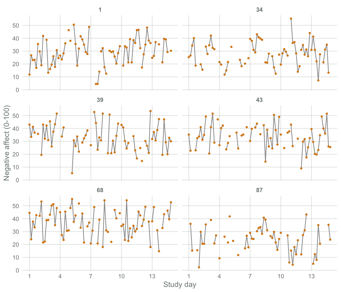
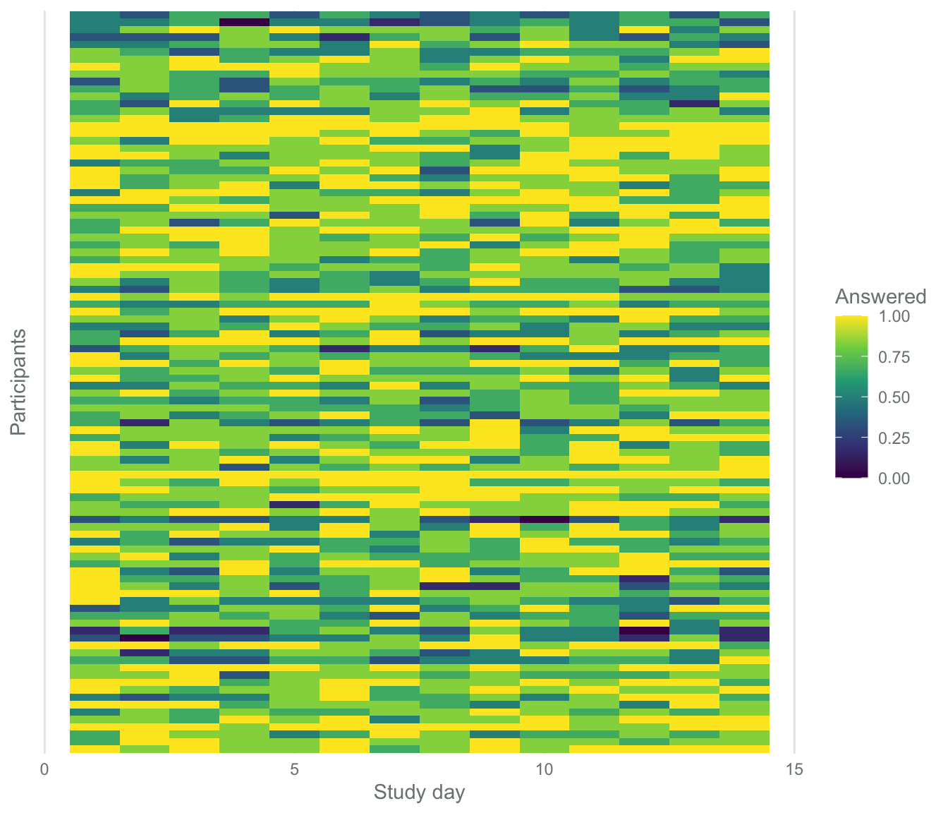
Plot individual time series for a random subset of participants, and plot compliance as a participant-by-day heat map. These plots can reveal flat-lining participants, technical outages, weekend effects, and trends that summary statistics hide.

library(ggplot2)

set.seed(1)
show_ids <- sample(unique(esm$id), 6)

esm |>
  filter(id %in% show_ids) |>
  mutate(study_time = day + (beep - 1) / 6) |>   # position within the 14 days
  ggplot(aes(study_time, na)) +
  geom_line(aes(group = day), colour = "grey60") +
  geom_point(size = 0.9, colour = "#D98A1F") +
  facet_wrap(~ id, ncol = 2) +
  scale_x_continuous(breaks = c(1, 4, 7, 10, 13)) +
  labs(x = "Study day", y = "Negative affect (0-100)") +
  theme_primer()

Figure 5.3: Negative affect for six randomly chosen participants. Lines connect prompts within the same day.

esm |>
  mutate(answered = !is.na(started)) |>
  group_by(id, day) |>
  summarise(prop = mean(answered), .groups = "drop") |>
  ggplot(aes(day, factor(id), fill = prop)) +
  geom_tile() +
  scale_fill_viridis_c(limits = c(0, 1)) +
  scale_y_discrete(breaks = NULL) +
  labs(x = "Study day", y = "Participants", fill = "Answered") +
  theme_primer()

Figure 5.4: Proportion of prompts answered per participant (rows) and study day (columns).

Delespaul, P. A. E. G. (1995). Assessing schizophrenia in daily life: The experience sampling method. Maastricht University Press.

Enders, C. K., & Tofighi, D. (2007). Centering predictor variables in cross-sectional multilevel models: A new look at an old issue. Psychological Methods, 12(2), 121–138. https://doi.org/10.1037/1082-989X.12.2.121

Geldhof, G. J., Preacher, K. J., & Zyphur, M. J. (2014). Reliability estimation in a multilevel confirmatory factor analysis framework. Psychological Methods, 19(1), 72–91. https://doi.org/10.1037/a0032138

Hamaker, E. L. (2012). Why researchers should think “within-person”: A paradigmatic rationale. In M. R. Mehl & T. S. Conner (Eds.), Handbook of research methods for studying daily life (pp. 43–61). Guilford Press.

Revol, J., Carlier, C., Lafit, G., Verhees, M., Sels, L., & Ceulemans, E. (2024). Preprocessing experience-sampling-method data: A step-by-step framework, tutorial website, R package, and reporting templates. Advances in Methods and Practices in Psychological Science, 7(4). https://doi.org/10.1177/25152459241256609